3D information can still be extracted from an image taken by an imaging device such as a camera. By knowing the physical processes that took place in converting a 3D information into a 2D. A location of an object in a real world can be represented by a three dimensional vector. However, in computer graphics, to further help the modeling of the object, the coordinates must need to be homogeneous. It is simply transforming a nx1 vector into an (n+1)x1 vector and multiplying the real world coordinates with the nth element. In the image space, since it is only limited to 2 dimensions, representing it in homogeneous coordinates will change it from a 2x1 vector into a 3x1. Since image representations of the real world are augmented vector space vectors, a non-linear relationship between the image location and the real world location can be obtain, and it is given by,

where Pi are the homogeneous coordinates of the object in the image, Pgo, on the other hand are the homogeneous coordinates of the object in the real world, and A is the transformation matrix, intrinsic to the imaging device, that involves a translation matrix, that gives the translation of the object origin of the real world coordinate system to the image plane origin, and a rotational matrix, that gives the rotational matrix needed to coincide the real world coordinate to the image-centric coordinate system.

From the equation given above, we can solve the image coordinate of a the object in terms of the the real world coordinates of the object. The image coordinates are given by,

Now by setting a34 = 1, we can separate the a's and solve through systems of linear equations. The separated a's are given by the equation,

From the equation above, for a single point in an image plane, we have 11 a's that are unknown. To solve this problem, we must have points greater than the number of unknowns.

In calibrating imaging device used in capturing the image, we used a Tsai grid, shown in Figure 1, to get the intrinsic a's.

Figure 1. Tsai grid used in calibrating the camera used in taking this picture.

The size of each square block are known, so from this image, we can get 11 real world points that specifies the xo, yo, and zo, and also from these points we can specify the image location. The previous equation can be represented by,

where Q is the left most matrix from the previous equation, a is the matrix of a's, and p is the right most matrix in the previous equation. The a's can be solved by the second equation showed above. To create Q, we must stack the left most matrix we obtained from each point. The same must be done to the right most matrix so that p can be constructed.

Now that we have the a's of the camera, we can now transform image coordinates to real world coordinates and vice versa. To test if the a's obtained are correct, a real world coordinate was picked and was then displayed on the image. Table 1 shows the real world coordinates used for the verification of the calibration and Figure 2 shows the transformed points.

Table 1. Real world coordinates and its corresponding image coordinates.

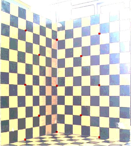
Figure 2. Tsai grid displayed with the transformed real world coordinates.

In summary of this article, we have calibrated an imaging device and verified if the calibration is correct by transforming a real world coordinate to an image coordinate.

Reference

• Dr. Soriano. Applied Physics 187 activity 8 manual.

Gamut gamut gamut!

Our eyes can only detect a finite number of colors. These colors are defined by the sensitivity of the cones in our eyes. One institution that defined these sensitivities is the International Commission on Illumination (CIE). The CIE Standard Human Observer is shown in Figure 1.

Figure 1. CIE standard human observer. The plot shows the sensitivities of each rod on different wavelengths in the visible region.

From these sensitivities, a color gamut can be constructed to show all the possible colors that can a standard human can observe. Using the equations below we can calculate the boundary of colors that a standard human eye can observe.

P is the emittance spectra of the light source and X, Y, and Z is the sensitivity of the three cones of a standard human eye. Here we used a Dirac delta function centered at each wavelength in the visible region. This will represent a light source that has a single and unique color. Applying this method we'll get the color gamut of a standard human observer shown in Figure 2.

Figure 2. Color gamut of a standard human observer.

The objective in this article is to show how large is the color gamut of a certain display and how compare it to the color gamut of a standard human eye.

To construct a gamut of a certain display, we will need to get the emittance spectra of it while displaying a red, green and blue color. This will replace the Dirac delta function we used for the P. Then we plot the x and y then plot it with the color gamut of a standard human eye.

We used a Toshiba laptop LCD and a Epson projector for the displays. We made it display a red, green, blue, white and black color.

Figure 3. Color gamuts of a Toshiba laptop LCD and Epson projector.

We can see that the color gamuts of both the laptop LCD and projector is smaller compared to the color gamut of a standard human observer. Also we can see that when both the displays are made to show a black and white color, it is located at the region where red, green and blue are equal in magnitudes.

In summary of this article, we have showed the boundary of colors that a standard human eye can observe. Also, color gamuts of two displays are compared to the standard human observer.

Reference

• Dr. Soriano. Applied Physics 187 activity 5 manual.
• http://www.cis.rit.edu/people/faculty/montag/vandplite/pages/chap_9/ch9p1.html
• http://hyperphysics.phy-astr.gsu.edu/hbase/vision/rodcone.html
• http://en.wikipedia.org/wiki/Gamut
• Chromaticity. Wikipedia: The Free Encyclopedia. http://en.wikipedia.org/wiki/Chromaticity.
• International Commission on Illumination. http://en.wikipedia.org/wiki/International_Commission_on_Illumination.
• CIE FREE DOCUMENTS FOR DOWNLOAD. http://www.cie.co.at/main/freepubs.html.

Light and Matter Relationship

Light and matter react with each other in different ways. Light, with its numerous wavelengths, travel in space and interact with anything it hits, mainly matter or another light. In general, light and matter interact with 3 ways, transmission, reflection and absorption. From this interaction and the rules of Physics, numerous phenomenons appear in the environment.

When considering these processes, we must look at the properties of light as a wave and matter in the atomic scale. Light waves have their corresponding wavelengths and intensity. This corresponds to a certain energy level. When looking at matter in the atomic scale, we know that atoms contain electrons in a certain orbital in reference to the nucleus. These orbitals have certain energy levels.

Let us consider a single wavelength light and a single atom with a single electron matter. Now, when light with the same energy level as the electron of a certain atom hits the matter, the energy of light is absorbed by the electron, the electron vibrates and releases the energy in other forms other than light (e.g. heat). Now, if the energies do not match, the electron will vibrate for a short period of time and release the energy in the form of light as well. If the object is transparent, the vibration is passed from atom to atom, and finally released on the other side. This corresponds to transmission. But if the object is opaque, electrons on the surface vibrates and releases light on the same side as the source, corresponding to reflectance. Now, if we scan the wavelength of light for the visible range, we can create a profile of how matter will react with light sources of different wavelengths.

Some samples in our everyday environment can demonstrate these processes.

Figure 1. Brightly Colored Leaf

Here we can see how absorption and reflection occurs in everyday objects. The brightly colored leaf reflects red to pink and absorbs the rest. This occurs in almost all objects. It can be also seen in the background image of the wall. The color we see is the reflected wavelengths while everything else is absorbed.

Now, reflection can be classified into 3 more sub-classifications, specular, body and interreflection. Specular reflection, also known as glossy reflection is the reflectance of almost the whole light source due to the angle of incidence. Body or matte reflection is the reflection after absorption has occurred. And interreflection is the reflection of light from a secondary object.

Figure 2. Reflection of the street on the side of a car

Figure 3. Reflection of light off a handkerchief to a wall

In figure 2, we can see all three types of reflection. First, lets examine the strip of metal on the side of the car. The different shades of silver shows the specular reflection (brightly colored silver) and the body reflection (slightly darker silver). Now, interreflection can be seen on the side of the car. Since the car paint is very glossy, the interreflection shows a clear image of the yellow line in the parking lot. Meaning light from the environment hits the yellow line, the yellow line reflects the colors it does not absorb to the car and the car reflects to the camera. This is slightly confusing, so lets take a look at figure 3. In figure three, we see the body reflection of the handkerchief as red and the body reflection of the wall as white. The interreflection can be seen as the red tinge on the wall coming from the red handkerchief.

Now, let us examine some images on transmission.

Figure 4. Transmission of light from an LED through a pane of glass

As discussed earlier, we can see that the transparent object transmitted the light from the side of the light source to the opposite side. Since the pane of glass is highly transparent for almost all wavelengths, we can see the light from the source very clearly and with the same color as the source. Now, most filters with certain colors reflect and transmit the same wavelengths. But there are some objects designed to transmit a different wavelength from the reflected wave.

Figure 5. Front view of a Dichroic Filter

Figure 6. Rear view of a Dichroic Filter

From the front (figure 5), we can see that the filter reflects almost all wavelengths with slight tinges of blue. This is the reflection part. From the rear (figure 6), we can see that the filter transmits red relatively more. This is very useful for museums and galleries where red light (longer wavelengths) can heat and damage the paintings.

Figure 7. Diffraction and interference of light through gratings

Now, let us consider a grating. A grating can be a transparent object with a series of evenly spaced opaque strips. When light hits an opaque strip, each point on the strip acts as a new source of light. When light transmits, light from each new point source interferes with each other producing either bright lights (constructive interference) or dark lights (destructive interference). From optics classes, we know that the equation for grating interference is as follows:

where d is the grating separation, theta m is the angle from the central axis, m is integer specifying the modes and lambda is the wavelength of the incident light. This determines the angles at which constructive interference occurs. As we can see, interference is dependent on the wavelength of light. This is because diffraction gratings are determined by the phase difference due to path difference to create constructive and destructive interference. As we can see in figure 7, light is diffracted differently per wavelength.

So how can we get the transmission, reflection and absorption profiles of different objects? All we need is the color signal of the object and the color signal of the light source on something white. The color signal of the object is thus the reflection of the object with the light source used. So by dividing the color signal of the object by the color signal of the light source on white. This will result to the reflection profile of the object. If we subtract that to 1 (when the reflection profile is normalized), will get the transmission/absorption profile. So how do we know if the profile we get is the absorption profile or the transmission profile? The simplest way to know is to look at the object. If the object is opaque, then it is the absorption profile. If the object is transparent, then the result is the transmission profile. So, lets look at different transmission and absorption of different objects.

Figure 7. Graph of Reflection and Absorption of a Black Wallet

Figure 8. Graph of Reflection and Absorption of a Blue BPI Card

Figure 9 Graph of Reflection and Absorption of a Green Mini-Guitar

Figure 10. Graph of Reflection and Absorption of a 5 Peso Coin

Figure 11. Graph of Reflection and Absorption of a 20 Peso Bill

Figure 12. Graph of Reflection and Absorption of a 100 Peso Bill

This can be verified by confirming the color of the object. We can see that the reflectance and absorption profiles correspond to the object colors. Also, we can see the limitations of the detector in the "noisy" part of the profiles. We can see distinguishable noise in the regions wavelength less than 400 nm and wavelengths greater than 650 nm.

References:

Wikipedia: The Free Encylopedia

The Physics Classroom